
In today's era of artificial intelligence, almost all learning models, decision systems, and business processes rely on "optimization." From the most basic linear regression to the most cutting-edge deep neural networks, from route planning for logistics delivery to asset allocation for financial investment, behind all of them is the repeated process of "finding the optimal solution." The so-called optimization algorithm refers to a mathematical method that, under given constraints, uses systematic search and iteration to make the value of the objective function reach the global minimum (or maximum) as much as possible. An optimization algorithm is a theoretical framework and also a set of engineering tools that can be directly put into practice. For AI beginners, mastering the basic concepts of optimization algorithms and common implementation methods is equivalent to having the key that enables models to "learn" and "improve."

Basic Concepts of Optimization Algorithms
The mathematical formulation of an optimization problem can usually be written as:

Among them,f(x) is the objective function (also called the loss function), which measures the quality of the solution x ;X is the solution space, that is, the set of all possible values;gi(x) are the constraints, the rules that the solution must satisfy.
In machine learning, the objective function is often the model's error on the training data or the negative log-likelihood, and the constraints may be regularization terms, parameter ranges, or business rules. The core task of an optimization algorithm is, under the premise of satisfying the constraints, to continuously update along some search strategy until the convergence criterion is met (such as the change in the objective function being below a threshold, the number of iterations reaching an upper limit, etc.).
Key Elements
- Search Direction: Determines which way to go at each step; common ones include the gradient direction, random perturbation direction, etc.
- Step Size (Learning Rate): Controls the movement magnitude of each step. If the step size is too large, it is easy to "skip over" the optimum; if the step size is too small, convergence is slow.
- Iteration Strategy: Includes fixed step size, decaying step size, momentum acceleration, etc., used to improve convergence speed and robustness.
Classification of Mainstream Optimization Algorithms
Gradient-Based Algorithms
Gradient-based algorithms are the most common and most intuitive optimization means. The core idea is: under the premise that the objective function is differentiable, move along the negative direction of the gradient, because the gradient points in the direction of the fastest increase of the function, and the negative gradient naturally points in the direction of the fastest decrease.
- Gradient Descent (GD): The most basic form, with the update rule . In the early days of deep learning, GD was still mainstream, but because each iteration requires traversing all training samples, the computational cost is extremely high.
- Stochastic Gradient Descent (SGD): Each time, only one sample or a mini-batch is used to estimate the gradient, greatly reducing the computational cost of a single iteration and making training on large-scale datasets possible.
- Momentum and Nesterov Accelerated Gradient: Add the "inertia" of historical gradients on top of SGD, helping the algorithm accelerate through steep valleys and avoid oscillating back and forth in narrow ravines.
- Adaptive Learning Rate Algorithms (AdaGrad, RMSProp, Adam): Dynamically adjust the learning rate by accumulating or exponentially decaying the historical gradient information of each parameter. Adam combines the advantages of momentum and RMSProp and has become one of the most commonly used optimizers in deep learning.
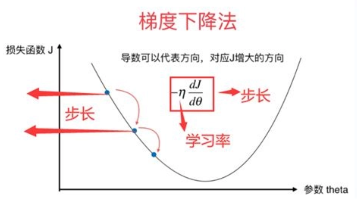
The advantage of gradient-based algorithms lies in their simple implementation and fast convergence speed (especially for adaptive methods such as Adam), but they require the objective function to be continuously differentiable, making them unsuitable for discrete combinatorial optimization or black-box function scenarios.
Second-Order and Quasi-Second-Order Methods
Second-order methods use the Hessian matrix of the objective function (i.e., the second derivative) to obtain a more precise search direction.
- Newton's Method: It directly uses the inverse of the Hessian to correct the gradient direction, and in theory can achieve quadratic convergence within one iteration.
- Quasi-Newton Methods (BFGS, L-BFGS): Without explicitly computing the Hessian, they approximate the Hessian by accumulating gradient changes, balancing the advantages of second-order information with acceptable computational cost.
Second-order methods perform excellently when the parameter dimension is not too high and the objective function is smooth. In deep learning, because model parameters often number in the millions or even hundreds of millions, the cost of computing the Hessian and its inverse is prohibitive, so second-order methods are more often used for fine-tuning small models or feature selection.
Metaheuristic (Evolutionary) Algorithms
When the objective function is non-differentiable, contains discrete variables, or the global optimum is distributed in an extremely complex way, traditional gradient-based methods often fail. In such cases, metaheuristic algorithms, through random search mechanisms that simulate natural or physical processes, can perform global exploration in a large solution space.
| Algorithm | Inspired by natural/physical phenomena | Basic process |
|---|---|---|
| Genetic Algorithm (GA) | Biological evolution (selection, crossover, mutation) | Initialize population → calculate fitness → selection → crossover → mutation → iterate |
| Particle Swarm Optimization (PSO) | Bird flock foraging | Initialize particles → update velocity/position → record individual/global best → iterate |
| Simulated Annealing (SA) | The cooling process of metal annealing | Random perturbation → accept worse solutions according to temperature → cool down → iterate |
| Ant Colony Optimization (ACO) | Ants leave pheromones while foraging | Construct solutions → update pheromones → iterate |
| Differential Evolution (DE) | Vector differences generate new candidate solutions | Mutation → crossover → selection |
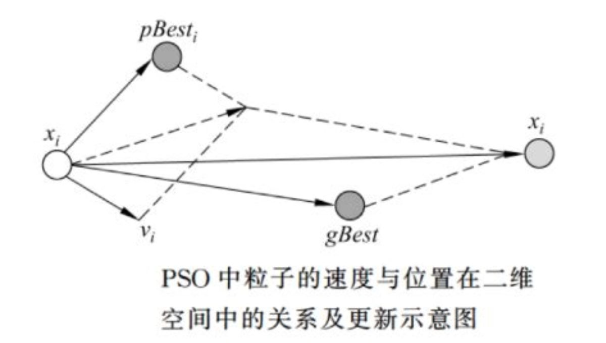
The common characteristic of these algorithms is that they do not rely on gradient information, so they can handle discrete, non-smooth, or even highly noisy objective functions. Their drawback is relatively slow convergence speed, and they require many hyperparameters to be tuned (population size, mutation probability, temperature decay rate, etc.).
Other Commonly Used Methods
- Conjugate Gradient: Suitable for solving large-scale linear systems, often used in quadratic optimization problems.
- Bayesian Optimization: By constructing a probabilistic model of the objective function (such as a Gaussian process), it selects the sampling point most likely to improve at each step, making it particularly suitable for global search of black-box functions, such as hyperparameter tuning for deep learning models.
- Policy Gradient in Reinforcement Learning: Treats the parameters of the policy as variables to be optimized, using gradient ascent (or descent) to increase cumulative reward.
Typical Applications of Optimization Algorithms in the AI Field
Training of Deep Neural Networks
In convolutional neural networks (CNNs), recurrent neural networks (RNNs), and the recent Transformer models, the training process is essentially a huge optimization problem of minimizing the cross-entropy loss. In most cases, researchers directly use Adam or SGD+Momentum for parameter updates.
- Advantages of Adam: The adaptive learning rate allows parameters in different layers to advance with appropriate step sizes, and it performs more robustly especially when the model structure is imbalanced (e.g., larger gradients in shallow layers and smaller gradients in deep layers).
- Advantages of SGD+Momentum: It can maintain better generalization ability on large-scale data, and especially when combined with cosine annealing of the learning rate, the model often achieves lower validation error.
Case: When using ResNet-50 for image classification on ImageNet, training with Adam (learning rate 1e-3) for 10 epochs improved Top-1 accuracy from 68% to 76%; if SGD+Momentum is used instead (learning rate 0.1, momentum 0.9), after 90 epochs the accuracy can be further improved to 78%, but the training time increases significantly.
Automatic hyperparameter tuning
Hyperparameters such as the model's learning rate, regularization coefficient, and network depth have a huge impact on final performance. The traditional approach is manual grid search or random search, which is inefficient.
- Bayesian optimization: By constructing a posterior distribution of the objective function, at each step it selects the most promising hyperparameter combination for experimentation, significantly reducing the number of experiments.
- Genetic algorithm: Each set of hyperparameters is encoded as a chromosome, and after selection, crossover, and mutation a new generation is produced, which can converge quickly in discrete search spaces (such as the number of layers and activation function types).
Combinatorial optimization and business decision-making
In industries such as logistics, manufacturing, and finance, common problems such as route planning, production scheduling, and asset allocation are essentially discrete combinatorial optimization.
- Simulated annealing: In the traveling salesman problem (TSP), by gradually lowering the temperature and accepting inferior solutions, it can escape local optima and obtain a route close to the global optimum.
- Ant colony algorithm: In the vehicle routing problem (VRP), the positive feedback mechanism of pheromones helps multiple vehicles collaboratively complete delivery tasks and significantly reduces total mileage.
- Particle swarm optimization: In the risk-return trade-off of financial investment portfolios, the global search capability of particle swarm is used to quickly locate asset allocation plans with controllable risk and relatively high return.
Model compression and quantization
Deploying models on mobile or embedded devices requires reducing model size while maintaining accuracy.
- Gradient descent + Lagrange multipliers: Adding sparse constraints during training gradually makes the weight matrix sparse, and ultimately model compression is achieved through pruning.
- Second-order information: Using a diagonal approximation of the Hessian to evaluate each parameter's sensitivity to the loss, important parameters are retained with priority and unimportant weights are discarded, achieving efficient quantization.
Practical guide: how to choose and tune parameters
Selection process (hierarchical decision-making)
- Determine differentiability
- Differentiable → prefer gradient-based methods (SGD, Adam).
- Non-differentiable or discrete → use metaheuristics (GA, PSO, SA).
- Evaluate scale and resources
- Parameters ≤ 10⁴ → consider second-order or quasi-second-order (BFGS, L-BFGS).
- Parameters ≥ 10⁶ → first-order or adaptive methods must be used.
- Constraint complexity
- Linear constraints → projected gradient or Lagrange multipliers.
- Nonlinear/mixed constraints → use the cross-entropy method or a hybrid evolutionary-gradient framework.
- Objective function characteristics
- High noise, black box → Bayesian optimization or simulated annealing.
- Multi-objective → use multi-objective evolutionary algorithms such as weighted sum or Pareto front (NSGA-II).
Key points of hyperparameter tuning
| Hyperparameter | Common value range | Tuning advice |
|---|---|---|
| Learning rate (LR) | 1e‑2 ~ 1e‑5 | Start large then decrease; for Adam, a starting point of 1e-3 is recommended; use warm-up + cosine annealing |
| Batch size (Batch) | 16 ~ 512 | Large batches improve parallelism; small batches add noise and help escape local optima |
| Momentum coefficient | 0.9 ~ 0.99 | Must be set for SGD; Adam has it built in |
| Population size (GA/PSO) | 30 ~ 200 | The larger the size, the more comprehensive the search, but the computational cost rises accordingly |
| Mutation rate (GA) | 0.01 ~ 0.1 | Moderate mutation prevents premature convergence and can be gradually reduced over iterations |
| Initial temperature (SA) | 10%–20% of the objective function magnitude | Too low a temperature leads to local search; too high a temperature leads to slow convergence |
Common pitfalls and avoidance strategies
- Vanishing/exploding gradients: Add Batch Normalization, residual connections to deep networks, or use gradient clipping (e.g.,
torch.nn.utils.clip_grad_norm_) to stabilize gradients. - Premature convergence: Use learning rate warm-up, noise injection (Dropout, random masking), or switch to adaptive optimizers such as Adam.
- Slow convergence of metaheuristics: First use GA to produce good initial solutions, then use gradient descent for local refinement; or adopt a hybrid evolutionary-gradient framework to achieve global exploration + local acceleration.
- Improper constraint handling: Use projection operators for hard constraints (e.g., project onto the feasible region), and use Lagrange multipliers or penalty functions for soft constraints, to avoid infeasible solutions during iteration.
Code example (Python)
Below is a typical Adam training loop example, suitable for most beginner projects. Learning rate decay and gradient clipping are added to the code to help beginners avoid common gradient problems.
import torch
import torch.nn as nn
import torch.optim as optim
from torch.utils.data import DataLoader

# 简单的全连接网络
class SimpleNet(nn.Module):
    def __init__(self, input_dim=784, hidden=256, output=10):
        super().__init__()
        self.net = nn.Sequential(
            nn.Linear(input_dim, hidden),
            nn.ReLU(),
            nn.Linear(hidden, output)
        )
    def forward(self, x):
        return self.net(x)

model = SimpleNet()
criterion = nn.CrossEntropyLoss()
optimizer = optim.Adam(model.parameters(), lr=1e-3)

# 学习率调度器:每 10 epoch 衰减 0.5
scheduler = optim.lr_scheduler.StepLR(optimizer, step_size=10, gamma=0.5)

for epoch in range(30):
    for xb, yb in DataLoader(train_dataset, batch_size=64, shuffle=True):
        xb = xb.view(xb.size(0), -1)          # 展平
        logits = model(xb)
        loss = criterion(logits, yb)

        optimizer.zero_grad()
        loss.backward()
        # 梯度裁剪,防止爆炸
        torch.nn.utils.clip_grad_norm_(model.parameters(), max_norm=5.0)
        optimizer.step()
    scheduler.step()
    print(f'Epoch {epoch+1:02d} - Loss: {loss.item():.4f}')
In the coming years, hybrid optimization frameworks (such as evolutionary-gradient and gradient-reinforcement learning) will become standard configurations, balancing global search and local acceleration. At the same time, the embedding of interpretability and safety constraints will enable optimization algorithms to gain regulatory recognition in key industries such as energy, transportation, and finance. As hardware accelerators efficiently support second-order information, quasi-second-order methods are expected to rise again in large model training. Bayesian optimization and automated hyperparameter search will further lower the barrier to AI development, realizing “one-click parameter tuning.” Overall, optimization algorithms will play an even more critical role in improving model performance, reducing resource consumption, and ensuring system reliability, driving AI technology to rapidly penetrate broader application scenarios.