
A neural network is a computational model built to mimic biological nervous systems. It processes information through layers of interconnected neurons and can learn complex patterns from data, making it one of the core technologies in the field of artificial intelligence.

Neural Network
What Is a Neural Network?
A neural network, whose full name isArtificial Neural Network(Artificial Neural Network, ANN), is a mathematical or computational model built to mimic the structure and function of biological neural networks (especially the brain). Its core idea is to estimate or approximate complex functions by simulating the connections and information transmission between biological neurons. A neural network consists of a large number of interconnected artificial neurons. The neurons are arranged in layers and transmit and process data based on weighted connections. Simply put, we can think of a neural network as a complex network composed of many small computational units (neurons). The computational units work together to accomplish specific tasks, such as recognizing images, understanding language, or predicting trends.
A neural network is a branch of machine learning and a core component of deep learning models . It learns patterns and relationships from training data, continuously adjusts and improves, and uses what it has learned to make predictions or decisions.
The design of neural networks is inspired by the network structure of neurons in the biological brain. They achieve intelligence by simulating the connections and information transmission processes between brain neurons. Neural networks learn how to perform tasks by analyzing large amounts of example data, and the learning process is similar to how humans accumulate knowledge through experience. For example, by showing a neural network tens of thousands of pictures of cats, it learns the features for recognizing cats and can identify cats in pictures it has never seen before.This learning ability has enabled neural networks to achieve great success in fields such as image recognition, speech recognition, and natural language processing, making them one of the important technologies driving the development of artificial intelligence.
Why Are Neural Networks So Important?
Neural networks are important becausethey have powerful learning and generalization capabilities. By learning from large amounts of data, they can automatically extract useful features and discover complex patterns hidden in the data without the need for manually written specific rules. This enables neural networks to perform exceptionally well when processing unstructured data such as images, speech, and text. For example, in image recognition tasks, neural networks can learn hierarchical features ranging from edges and textures to object parts, achieving high-precision recognition.Neural networks have a high degree of parallel processing capability. A large number of neurons in the structure can perform computations simultaneously, enabling efficient processing of large-scale datasets and achieving significant acceleration on modern parallel computing hardware (such as GPUs).
Neural networks are the core of modern artificial intelligence, especially deep learning. Deep learning models, such as Convolutional Neural Networks (CNNs) and Recurrent Neural Networks (RNNs), are essentially deep neural networks with specific structures, and they have achieved breakthrough progress in fields such as computer vision, natural language processing, and speech recognition. For example, large language models (such as ChatGPT) and AI image generators (such as DALL-E) rely heavily on neural network technology. Another important characteristic of neural networks isadaptability. Based on adjusting hyperparameters such as network structure, activation functions, and loss functions, as well as adopting different training strategies, neural networks can be applied to a variety of different tasks, including classification, regression, clustering, generation, and more. This flexibility makes neural networks a general framework for solving various real-world problems.
Neurons
Biological Neurons and Artificial Neurons
To understand artificial neural networks, it is necessary to understand their source of inspiration—biological neurons. Biological neurons are the basic units that make up the animal brain and nervous system, processing and transmitting information based on complex connection networks. A typical biological neuron mainly consists ofthe cell body, dendrites, and axonthree parts.Dendritesare numerous branch-like structures extending outward from the cell body, responsible for receiving electrical signals from other neurons or the external environment.The cell bodyis the core of the neuron, responsible for integrating and processing the received signals. When the signal strength received by the cell body accumulates beyond a certain threshold, the neuron is activated and generates an electrical impulse (action potential). The electrical impulse is transmitted based onthe axon—a relatively long fiber extending from the cell body. At the end of the axon there are many axon terminals, which form connection points with the dendrites of other neurons, calledsynapses . Neurotransmitters are released from the axon terminal of one neuron based on the synapse and transmitted to the dendrites of the next neuron, thereby achieving information transmission between neurons.
Artificial neurons, also callednodesorunits, are a simplification and simulation of biological neurons. They have the function of receiving input, processing information, and producing output. The input of an artificial neuron (similar to the dendrites of a biological neuron) can be one or more numerical values, and each input carries aweight, representing the importance or strength of the input. Inside the neuron, all weighted inputs are summed, and abias term(bias) is added. The weighted sum is then sent to an activation function for processing. The role of the activation function is similar to the threshold mechanism of a biological neuron, determining whether the neuron is activated and the degree of activation, and passing the processed result as the output of the neuron (similar to the axon of a biological neuron) to the next layer or other neurons.
The Hierarchical Structure of Neural Networks
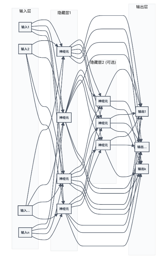
The key to neural networks being able to handle complex tasks lies in a carefully designed hierarchical structure, allowing the network to gradually extract useful features from raw input data and output meaningful results. A typical neural network contains three types of layers:the input layer, hidden layers, and output layer . Each layer consists of several parallel neurons (or nodes), and neurons are the basic units for computation and information processing in the network. Layers are associated with one another through weighted connections, and the weights determine the strength and influence of signals when transmitted between layers.Information flows in one direction in the network, starting from the input layer, passing forward layer by layer, undergoing processing by one or more hidden layers, and finally reaching the output layer to obtain the network's prediction or classification result.
Input Layer
The input layer is the starting point of a neural network, and it is also the only layer that directly interacts with external data. It mainly receives raw input data and passes it to subsequent hidden layers in a form that the network can understand and process. Each neuron in the input layer corresponds to one feature in the input data.
For example, when processing image data, if the image is a 28×28 pixel grayscale image, the input layer may contain 784 neurons, each representing the grayscale value of one pixel. If the image is color and uses RGB mode, each pixel will be represented by values from the red, green, and blue channels, and the number of neurons in the input layer will be the product of the image width, height, and number of channels (for example, 28x28x3).
For tabular data, each column usually represents one feature, and the number of neurons in the input layer is equal to the number of columns in the table (that is, the number of features). Importantly,the input layer itself does not perform any computation or transformation operations, and only passes the received raw data unchanged to the next layer.
The design of the input layer depends directly on the dimensions and type of the input data. Ensuring that the data enters the network accurately and without error is the foundation for all subsequent computation and analysis.
Hidden Layers
Hidden layers are one or more intermediate layers located between the input layer and the output layer in a neural network, and they are the core of the neural network's complex computations and feature learning. They are called “hidden layers” because the outputs of the layers are not directly exposed to the outside world, but instead serve as part of the network's internal state, used to gradually abstract and extract high-level features from the input data. A neural network may have no hidden layers (such as a single-layer perceptron), or it may have one or more hidden layers.The number of hidden layers and the number of neurons in each hidden layer (that is, the width and depth of the network) are key hyperparameters of a neural network, and they directly determine the network's complexity and learning ability.
Output Layer
The output layer is the last layer of the neural network, and its main function is to aggregate the information after processing and transformation by all the preceding hidden layers and generate the final output result, which is the neural network's prediction or classification of the input data. The number of neurons in the output layer and the type of activation function used depend on the specific type of problem to be solved. For example, inbinary classification problems(such as determining whether an email is spam), the output layer contains only one neuron and uses Sigmoid as the activation function, and the output value of the neuron can be interpreted as the probability of belonging to a certain category. Formulticlass classification problems(such as handwritten digit recognition, with 10 categories in total), the output layer contains the same number of neurons as the number of categories (for example, 10 neurons) and uses the Softmax activation function. The Softmax function can convert the output of each neuron into the probability of the corresponding category and ensure that the sum of the probabilities of all categories is 1.
Forregression problems(such as predicting house prices), the output layer has only one neuron and generally does not use an activation function, or uses a linear activation function, directly outputting a continuous numerical value as the prediction result. In some complex regression tasks, for example, when it is necessary to simultaneously predict the coordinates and size of an object's bounding box, the output layer contains multiple neurons (for example, 4, corresponding to the height, width, x-coordinate, and y-coordinate of the bounding box), and each neuron outputs a continuous numerical value.The design of the output layer is directly related to whether the network can give meaningful predictions that meet the requirements of the problem. When choosing the structure of the output layer and the activation function, the nature and goal of the task must be fully considered.
How Do Neural Networks Learn?
Forward Propagation
Forward Propagation is the core process by which a neural network makes predictions or computations, describing how input data starts from the input layer, is passed forward layer by layer, and finally reaches the output layer and produces an output result. This process is the foundation for a neural network to learn and work. The raw input data is fed into the various neurons of the input layer. The neurons of the input layer simply pass the data (for example, the pixel values of an image or the word vectors of text) to the neurons of the next layer (usually the first hidden layer).
In each neuron of the hidden layers and the output layer, a series of standard computation steps is performed. Taking the j-th neuron of layer l as an example, it receives the outputs of all neurons in the previous layer (layer l-1) (denoted as aᵢˡ⁻¹) as input. Each input aᵢˡ⁻¹ is multiplied by a corresponding connection weight wᵢⱼˡ (representing the connection weight from the i-th neuron of layer l-1 to the j-th neuron of layer l). The neuron sums all weighted inputs and adds a bias term bⱼˡ specific to that neuron. The result of the weighted sum plus the bias term is denoted as zⱼˡ = Σᵢ (wᵢⱼˡ * aᵢˡ⁻¹) + bⱼˡ. The intermediate result zⱼˡ is fed into a nonlinear activation function g(·), yielding the final output of the neuron aⱼˡ = g(zⱼˡ). The output aⱼˡ serves as the input to the neurons of the next layer, or if the current layer is the output layer, aⱼˡ is one of the final outputs of the network.
This process is repeated in the network starting from the input layer, moving forward layer by layer (toward the output layer), until the output values of all neurons in the output layer are computed. The outputs of the output layer constitute the neural network's prediction result for the current input sample. For example, in an image classification task, each neuron in the output layer represents a category, and the output value indicates the probability that the input image belongs to that category.The forward propagation process is deterministic, once the network's weights and biases are determined, given an input, the output is uniquely determined. During the training process of a neural network, forward propagation is an indispensable step because it produces the network's predictive output, and the output will be used to compare with the true labels, calculate the loss function, and guide the updating of the network parameters.
Loss Function
The loss function(Loss Function), also called the cost function (Cost Function) or objective function (Objective Function), is a crucial component in the training process of a neural network. Its core role is toquantify the degree of difference or "error" between the neural network's predicted output on a given training sample and the true label (or expected output) . The smaller the value of the loss function, the closer the neural network's prediction is to the true situation, and the better the model's performance. Therefore,the goal of training a neural network is to minimize the value of the loss function by adjusting the network's parameters (weights and biases) 。
Which loss function to choose depends on the specific task type. The following table summarizes some common loss functions and their main characteristics:
| Task Type | Loss Function Name | Mathematical Expression (Simplified Version) | Main Characteristics |
|---|---|---|---|
| Regression Problems | Mean Squared Error (MSE) | (1/N) * Σ(y_pred - y_true)² |
Gives larger penalties to larger errors, commonly used |
| Mean Absolute Error (MAE) | (1/N) * Σ|y_pred - y_true| |
Less sensitive to outliers than MSE | |
| Classification problems | Binary Cross-Entropy (Binary CE) | -[y_true * log(y_pred) + (1-y_true) * log(1-y_pred)] |
Used for binary classification tasks, measures the difference between probability distributions |
| Categorical Cross-Entropy (Categorical CE) | -Σᵢ (y_trueᵢ * log(y_predᵢ)) |
Used for multi-class classification tasks, y_true is usually one-hot encoded |
Table 1: Common loss functions and their main characteristics
The choice of loss function directly affects the model's training effectiveness and generalization ability. A good loss function can accurately reflect the degree of error in the model's predictions and has good mathematical properties during optimization (such as differentiability, so that gradient descent can be performed). During the training process of a neural network, after each forward pass produces the predicted output, the value of the loss function is calculated. The loss value then serves as the starting point of the backpropagation algorithm, used to guide the update of the network parameters, reducing the loss in the next iteration and improving prediction accuracy.
Backpropagation
The backpropagation algorithm is the core algorithm for training neural networks, especially multilayer perceptrons (MLPs), used to efficiently calculate the gradient of the loss function with respect to each parameter in the network. The gradient information is used by optimization algorithms (such as gradient descent) to update the network's weights and biases, gradually reducing prediction errors and improving model performance. The core idea of backpropagation isto start from the output layer based on the chain rule and calculate the partial derivatives of the loss function with respect to each weight and bias layer by layer backward。
The specific steps are as follows:
- Forward propagation to compute the output: Based on one complete forward pass, input a batch of training data into the network and compute the network's output.
- Compute the loss function: Compare the network's output with the true labels (target values) corresponding to the training data, and use a predefined loss function to calculate the network's prediction error.
- Compute the error term of the output layer: The first step of backpropagation is to calculate the partial derivative of the loss function with respect to the net input zj of each neuron j in the output layer, called the error term δj of that neuron. For an output layer neuron, δj = ∂L/∂aj · ϕ′(zj), where L is the loss function, aj is the neuron's output, and ϕ′(zj) is the derivative of the activation function at its net input zj.
- Backpropagate the error term: Once the error term of the output layer is calculated, propagate the error term backward through the network to the preceding hidden layers. For neuron j in hidden layer l, the calculation of the error term δjl depends on the error terms δkl+1 of all neurons k connected to it in the next layer (i.e., layer l+1) and the connection weights wjk between them. The specific formula is δjl = ϕ′(zjl) ∑k wjk δkl+1. Here zjl is the net input of neuron j in layer l.
- Compute the gradients of the parameters: After the error term δj of each neuron has been calculated, one can easily compute the gradient of the loss function with respect to each weight wij (connecting the i-th neuron to the j-th neuron) and each bias bj. For the weights, ∂L/∂wij = ai δj (where ai is the output of the previous neuron i). For the biases, ∂L/∂bj = δj.
- Update the parameters: Using the computed gradients, combined with an optimization algorithm (such as gradient descent), update all parameters in the network. For example, for a weight wij, the update rule is wij=wij−η∂wij∂L, where η is the learning rate, which controls the step size of parameter updates.
Optimizer
After the backpropagation algorithm computes the gradient of the loss function with respect to each parameter,optimizer(Optimizer) is tasked with updating the network's weights and biases based on gradient information to minimize the loss function. Think of the optimizer as a "navigator" that guides the direction of parameter optimization. The simplest optimizer isgradient descent (Gradient Descent, GD), which directly updates parameters along the negative direction of the gradient, with the update rule: parameter = parameter – learning rate * gradient. The learning rate (Learning Rate) is a very important hyperparameter that controls the step size of each parameter update.learning rateIf it is too large, the algorithm may oscillate or even diverge near the optimum; if the learning rate is too small, convergence may be too slow.
Standard gradient descent has some limitations, such as getting stuck in local optima, or slow convergence when the gradients differ greatly in different directions of the parameter space. To address these issues, researchers have proposed many more advanced optimization algorithms. The following table summarizes some common optimizers and their characteristics:
| Optimizer Name | Main Characteristics | Advantages | Disadvantages |
|---|---|---|---|
| Stochastic Gradient Descent (SGD) | Uses one training sample (or a small batch of samples) at a time to compute gradients and update parameters. | Fast computation, can escape certain local optima. | The update direction is unstable, and the convergence process may oscillate. |
| Momentum Method (Momentum) | Introduces a momentum term, simulating the concept of momentum in physics, accelerating SGD's convergence in relevant directions and suppressing oscillations. | Accelerates convergence and reduces oscillations. | Requires tuning the momentum hyperparameter. |
| AdaGrad | Adaptively assigns different learning rates to each parameter, using a larger learning rate to update parameters corresponding to less frequent features. | Suitable for handling sparse data. | The learning rate decreases monotonically, which may stop learning too early. |
| RMSProp | Improves AdaGrad by introducing a decay factor, accumulating only the squared gradients from a recent period, solving the problem of the learning rate decreasing too early. | Solves the problem of AdaGrad's learning rate dropping sharply. | Still requires manually setting the global learning rate. |
| Adam (Adaptive Moment Estimation) | Combines the ideas of the momentum method and RMSProp, simultaneously computing the exponential moving averages of the first moment (mean) and second moment (uncentered variance) of the gradients. | Generally performs well, is relatively robust to hyperparameter choices, and is one of the most widely used optimizers today. | Slightly higher computational overhead. |
Table 2: Common optimizers and their characteristics
Choosing the appropriate optimizer and its hyperparameters (such as the learning rate) is crucial for the training efficiency and final performance of neural networks. In practice, the Adam optimizer is widely used due to its good default performance and low need for hyperparameter tuning.
Types of Neural Networks
Common Types of Neural Networks
Neural networks are not a single structure; many diverse types have been developed to meet the needs of different tasks.
| Neural Network Type | Main Features | Typical Application Areas |
|---|---|---|
| Multilayer Perceptron (MLP) | The most basic feedforward neural network, comprising an input layer, one or more hidden layers, and an output layer, with full connections between layers. | Basic tasks such as classification and regression |
| Convolutional Neural Network (CNN) | Designed specifically for processing grid-like data (such as images), it uses convolutional layers and pooling layers to extract local features and has the characteristics of parameter sharing and sparse connectivity. | Image recognition, object detection, image segmentation, video analysis |
| Recurrent Neural Network (RNN) | Designed specifically for processing sequential data (such as text and speech), it has a recurrent structure that can pass information from the previous moment to the current moment. | Natural language processing (text generation, machine translation), speech recognition |
| Long Short-Term Memory Network (LSTM) | An improved type of RNN that effectively solves the vanishing/exploding gradient problem of RNNs by introducing a gating mechanism (input gate, forget gate, output gate), enabling it to learn long-term dependencies. | Tasks that need to handle long-sequence dependencies, such as machine translation and speech recognition |
| Gated Recurrent Unit (GRU) | Similar to LSTM, but with a simpler structure, having only an update gate and a reset gate, and usually with higher computational efficiency. | Similar to LSTM, performing comparably or better on some tasks |
| Autoencoder | An unsupervised learning network that encodes input data into a low-dimensional representation and then decodes it to reconstruct the original data, used for feature extraction and dimensionality reduction. | Data dimensionality reduction, feature extraction, anomaly detection, image denoising |
| Generative Adversarial Network (GAN) | Contains a generator network and a discriminator network, which learn through mutual competition; the generator tries to generate realistic data, and the discriminator tries to distinguish real data from generated data. | Image generation, image-to-image translation, data augmentation, super-resolution |
Table 3: Common neural network types and their features and applications
Overview of Neural Network Applications
Examples of Neural Networks in Real Life
Neural networks have penetrated every aspect of our daily lives. The following are some specific examples of neural networks in real life:

With the continuous advancement of technology, neural networks will play an important role in more fields in the future, changing the way we live and work.
Summary and Outlook
Advantages and Limitations of Neural Networks
As a powerful machine learning model, neural networks have significant advantages, but also limitations.
Advantages:
- Powerful nonlinear modeling capability: Based on the stacking of multiple layers of nonlinear activation functions, neural networks can learn and represent highly complex nonlinear relationships.
- Automatic feature extraction: Unlike traditional machine learning methods that require manually designed features, neural networks (especially deep learning models) can automatically learn useful feature representations from raw data, reducing manual intervention.
- Good generalization ability: When sufficient training data is available, a well-trained neural network can make accurate predictions on unseen data, demonstrating good generalization performance.
- Parallel processing capability: Neural network computation is based on a high degree of parallelization, which enables them to fully utilize hardware acceleration such as modern GPUs and efficiently process large-scale datasets.
- Wide range of application areas: Neural networks have been successfully applied in numerous fields such as computer vision, natural language processing, speech recognition, recommendation systems, medical diagnosis, and financial risk control, and have achieved breakthrough progress.
Limitations:
- Strong data dependence: Neural networks require a large amount of labeled data for training in order to achieve good performance. In scenarios with sparse data or high labeling costs, their application is limited.
- High computational resource consumption: Training deep neural networks requires powerful computational resources (such as high-performance GPUs) and long training times.
- Poor interpretability (black-box problem): The decision-making process of neural networks is often difficult to explain, and it is hard for people to understand exactly how the model makes a particular prediction internally, which limits their application in some high-risk fields (such as healthcare and finance).
- Prone to overfitting: When the model is too complex or the training data is insufficient, neural networks tend to perform well on the training set but poorly on the test set, that is, overfitting occurs. Techniques such as regularization and Dropout are needed to alleviate this.
- Difficult hyperparameter tuning: The performance of neural networks is very sensitive to hyperparameters such as network architecture, learning rate, and optimizer choice, and finding the optimal hyperparameter combination often requires a large amount of experimentation and experience.
- Vulnerability to adversarial examples: Neural networks are easily deceived by carefully designed tiny perturbations (adversarial examples), leading to incorrect outputs.
Future development trends
As the core driving force of artificial intelligence, neural networks have a future full of opportunities and challenges. The following directions deserve attention:
- More efficient and lightweight models: Future research will pay more attention to techniques such as model compression, knowledge distillation, network pruning, and quantization to build smaller, faster, and more energy-efficient models.
- Improving model interpretability and robustness: To solve the "black box" problem of neural networks and enhance credibility in critical fields, explainable artificial intelligence (XAI) will continue to receive attention. Improving model robustness to noise, outliers, and adversarial attacks is also an important research direction.
- Few-shot learning and self-supervised learning: To reduce dependence on large-scale labeled data, techniques such as few-shot learning, zero-shot learning, and self-supervised learning will be further developed, enabling models to learn from a small amount of data or even unlabeled data.
- Integration of neuro-symbolic AI: Combining the pattern recognition ability of neural networks with the logical reasoning ability of symbolic reasoning is expected to create more powerful AI systems that are closer to human intelligence.
- Continual Learning and Lifelong Learning: Future research will be dedicated to developing Continual Learning and Lifelong Learning algorithms that can continuously learn new knowledge and avoid catastrophic forgetting.
- Brain-inspired Computing and Neuromorphic Computing: Drawing on the more refined structure and working principles of the biological brain, design more efficient neural network architectures and computing paradigms, such as Spiking Neural Networks (SNNs) and neuromorphic chips, to achieve breakthroughs in energy efficiency and intelligence levels.
- AI Ethics and Safety: In the future, it is necessary to establish sound laws, regulations, and technical standards to ensure the healthy development of AI technology and prevent potential risks.