
Introduction: Understanding model training with a vivid analogy
Imagine you are a student preparing for a final exam, and your "model" is your brain. Your goal is not only to achieve good results on practice problems (training data), but also to perform well on the actual final exam (new data). In this process, you may encounter two extreme situations:
- Underfitting : This is like only roughly flipping through the textbook before an exam, without even mastering the most basic concepts and formulas. As a result, whether on practice problems or on the final exam, your scores are low. Your brain (model), because it is too simple, has not learned the essence of the data.
- Overfitting : This is equivalent to memorizing every question in the workbook, including the answers and solution steps, and even the stains next to the questions. You can get full marks when doing practice problems, but as soon as the final exam comes and the questions change slightly, you are at a loss. Your brain (model), because it is too complex, has not only learned the knowledge but also learned the "noise" and irrelevant details specific to the practice problems, resulting in extremely poor generalization ability.
This article systematically introduces the causes of these two problems, how to diagnose them, and provides a series of practical and easy-to-understand solutions, including code examples that can be used directly, to help you train an ideal model that is both smart and does not "rote-memorize."
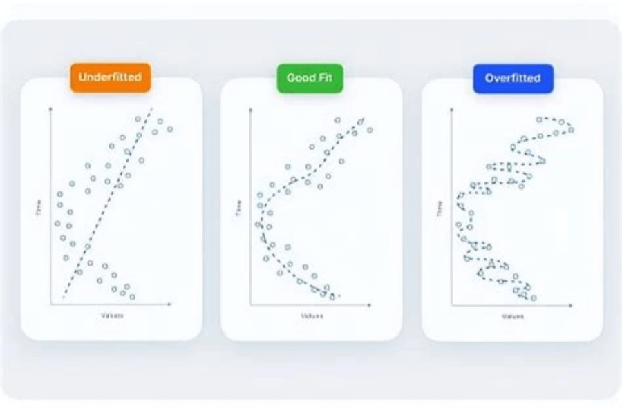
Core concepts: The tradeoff between bias and variance
To deeply understand underfitting and overfitting, you must first understand two core concepts: bias and variance. These two are the main sources of model error.
- Bias : Bias measures the systematic gap between the model's prediction results and the true results.High biasmeans the model is too simple and cannot capture the complex patterns in the data, directly leading tounderfitting . It is like a student who only knows addition being asked to do calculus; the answer he gives (prediction) will systematically deviate from the correct answer.
- Variance : Variance measures the stability and fluctuation of the model's prediction results when facing different training datasets.High variancemeans the model is too complex and sensitive, and will also treat random noise in the training data as patterns to learn, directly leading tooverfitting . It is like that "rote-memorizing" student: switch to another set of practice problems, and his answers will be worlds apart.
In machine learning, bias and variance are often a pair of contradictions, known as the "bias-variance tradeoff". A powerful, complex model (such as a deep neural network) has the ability to learn very fine-grained patterns, so its bias is low, but it is also more likely to learn noise, resulting in high variance. Conversely, a simple model (such as linear regression) has high bias but is less sensitive to changes in the data, so its variance is low. Our ultimate goal is to find the best balance between bias and variance so that the model's overall error is minimized.
How to diagnose problems: Learn to read the "learning curve"
Before taking action to solve the problem, we need a diagnostic tool to determine where the model is actually "sick."Learning curve is a very intuitive tool. By plotting the model's performance on the training set and validation set (a portion of data not involved in training, used to simulate a real exam), such as loss or accuracy, over the course of training (such as training epochs epochs), the curves of change reveal the model's learning state.
- Diagnosing underfitting: If both the training loss and validation loss are very high and eventually stabilize at a high level, it means the model is underfitting. The two curves are very close, indicating that the model cannot even learn the training data well, let alone generalize.
- Diagnosing overfitting: If the training loss continues to decrease and performs excellently, while the validation loss begins to rise after decreasing to a certain point, this is a typical signal of overfitting. A huge "gap" appears between the two curves, indicating that the model is "overly" familiar with the training data but performs poorly on new data.
- Ideal state: Both the training loss and validation loss steadily decrease and eventually converge to a low level, with the two curves close together. This indicates that the model has found a good balance point.
Strategies for solving "learning too shallowly": underfitting
When a model exhibits underfitting, our main goal is to enhance the model's learning ability.
Strategy 1: Increase model complexity
This is the most direct method. If a simple linear model cannot fit nonlinear data, we need a more powerful model.
- For traditional machine learning: You can try using more complex models, such as switching from linear regression to polynomial regression, support vector machines (using a Gaussian kernel), or gradient boosting trees.
- For neural networks: You can increase the number of layers in the network or the number of neurons in each layer.
Hands-on code: Using polynomial features to increase model complexity
The following Python code uses thescikit-learnlibrary to demonstrate how to make a simple linear model more powerful by adding polynomial features, thereby solving the underfitting problem.
import numpy as np
import matplotlib.pyplot as plt
from sklearn.pipeline import make_pipeline
from sklearn.linear_model import LinearRegression
from sklearn.preprocessing import PolynomialFeatures# 1. Create some nonlinear sample data that a linear model will struggle to fit
np.random.seed(0)
X = np.random.rand(30, 1) * 10
y = np.sin(X).ravel() + np.random.randn(30) * 0.5
X_test = np.linspace(0, 10, 100)[:, np.newaxis]# 2. Try using a simple linear model (1st-degree polynomial) to fit, which will cause underfitting
model_underfit = LinearRegression()
model_underfit.fit(X, y)# 3. Use a more complex model: 4th-degree polynomial regression
# PolynomialFeatures(degree=4) will transform the original feature X into [1, X, X^2, X^3, X^4]
# This greatly increases the model's complexity, enabling it to capture nonlinear relationships [[124]][[126]]
model_goodfit = make_pipeline(PolynomialFeatures(degree=4), LinearRegression())
model_goodfit.fit(X, y)# 4. Visualize the results
plt.figure(figsize=(10, 6))
plt.scatter(X, y, label='Sample Data')
plt.plot(X_test, model_underfit.predict(X_test), label='Linear Fit (Underfitting)', color='red')
plt.plot(X_test, model_goodfit.predict(X_test), label='4th-Degree Polynomial Fit (Good Fit)', color='green')
plt.title('Solving Underfitting by Increasing Model Complexity')
plt.xlabel('Feature')
plt.ylabel('Target Value')
plt.legend()
plt.show()
Strategy 2: Add more effective features (feature engineering)
Sometimes a model performs poorly not because it is not complex enough, but because the "raw materials" (features) provided to it contain insufficient information. Through Feature Engineering , we can create new features with greater value. For example, when predicting housing prices, in addition to "house area," we can also calculate "house age" from the "year built," or calculate the "distance from the city center" from geographic coordinates. These new features may contain stronger predictive signals.
Strategy 3: Reduce Regularization
Regularization is used to prevent overfitting (described in detail below), but if the strength of regularization is too high, it will overcorrect, excessively restricting the model's learning ability and leading to underfitting. If you find that the model is underfitting and you have used regularization, you can try reducing the regularization parameter.
Addressing "rote memorization": Strategies for Overfitting
Overfitting is the most commonly encountered problem in machine learning practice. Fortunately, we have a rich "arsenal" to deal with it.
Strategy 1: Increase Data Volume and Data Augmentation
Obtaining more datais the most fundamental and effective way to solve overfitting. The more data there is, the better the model can learn universal patterns from it, rather than being limited to the noise of specific samples.
In reality, obtaining new data is costly. Data Augmentation has therefore become a cost-effective choice. By making small, reasonable transformations to existing data, new training samples are created.
- For image data: operations such as random rotation, cropping, flipping, scaling, and adjusting brightness and contrast can be performed.
- For text data: synonym replacement, random insertion, or deletion of words can be performed.
Through data augmentation, we greatly enrich the diversity of the training data, forcing the model to learn more robust features.
Strategy 2: Regularization
The core idea of regularization is to add a "penalty term" to the model's loss function (the metric measuring prediction error). This penalty term is used to limit the model's complexity. While striving to reduce prediction error, the model must maintain its own "simplicity," thereby avoiding overfitting.
The two most common regularization methods are L1 and L2 regularization:
- L2 Regularization (Ridge Regression) : penalizes the sum of squares of the model weights (parameters). It tends to make all weights very small, but not exactly zero. This makes the model's decision-making process more "smooth" and less susceptible to drastic influence from a single data point.
- L1 Regularization (Lasso Regression) : penalizes the sum of the absolute values of the model weights. It has an interesting property: it tends to compress the weights of some less important features directly to zero, thereby achieving automatic Feature Selection 。
Hands-on Code: Using L2 Regularization to Mitigate Overfitting
The following Python code demonstrates how, in a scenario prone to overfitting, L2 regularization (inscikit-learnthrough theRidgeclass implementation) can effectively improve the model's generalization ability.
import numpy as np
import matplotlib.pyplot as plt
from sklearn.linear_model import LinearRegression, Ridge
from sklearn.preprocessing import PolynomialFeatures
from sklearn.pipeline import make_pipeline# 1. Create a small amount of complex sample data, which can easily lead to overfitting
np.random.seed(0)
X = np.random.rand(10, 1) * 10
y = np.sin(X).ravel() + np.random.randn(10) * 0.2
X_test = np.linspace(0, 10, 100)[:, np.newaxis]# 2. Use a very complex model (10th-degree polynomial) to fit, which will cause overfitting
model_overfit = make_pipeline(PolynomialFeatures(degree=10), LinearRegression())
model_overfit.fit(X, y)# 3. Apply L2 regularization (Ridge) on an equally complex model
# alpha is the regularization strength; the larger alpha is, the heavier the penalty [[63]]
model_regularized = make_pipeline(PolynomialFeatures(degree=10), Ridge(alpha=1.0))
model_regularized.fit(X, y)# 4. Visualize the results
plt.figure(figsize=(10, 6))
plt.scatter(X, y, label='Sample data')
plt.plot(X_test, model_overfit.predict(X_test), label='10th-degree polynomial fit (overfitting)', color='red')
plt.plot(X_test, model_regularized.predict(X_test), label='Fit with L2 regularization (better generalization)', color='green')
plt.title('Solving overfitting with L2 regularization')
plt.xlabel('Feature')
plt.ylabel('Target value')
plt.ylim(-2, 2)
plt.legend()
plt.show()
Strategy 3: Dropout (random deactivation)
Dropout is a very powerful and simple regularization technique in deep learning. Its way of working is much like an efficient team collaboration: at every step of model training, a portion of neurons is randomly "frozen" (or "dropped"), so that they do not participate in that computation.
This brings two benefits:
- Forces the network to learn redundant representations: Because any neuron may be "absent" at any time, the network cannot overly rely on a few specific neurons and must learn more robust and more distributed feature representations.
- Ensemble effect: From the perspective of the effect, each Dropout is equivalent to training a different, smaller subnetwork. The entire training process is like training thousands of different networks simultaneously and finally ensembling their results, which greatly enhances the model's generalization ability.
Strategy 4: Early Stopping
This is a very intuitive and effective "braking" mechanism. While training the model, we monitor the model's performance on the validation set in real time. Once we find that the loss on the validation set no longer decreases, or even begins to rise, we immediately stop training.
The benefit of doing this is that we can stop in time at the critical point when the model shifts from "learning knowledge" to "rote memorization", thereby obtaining a model with generalization ability close to the best.
Hands-on code: Using Early Stopping in Keras
The following code shows how to easily implement early stopping in the deep learning framework Keras.
# Assume we have already imported the necessary libraries and prepared the training data (X_train, y_train) and validation data (X_val, y_val)
# from keras.models import Sequential
# from keras.layers import Dense
# from keras.callbacks import EarlyStopping# 1. Define a simple neural network model
# model = Sequential()
# model.add(Dense(128, activation=’relu’, input_dim=…))
# model.add(Dense(64, activation=’relu’))
# model.add(Dense(1, activation=’sigmoid’))
# model.compile(optimizer=’adam’, loss=’binary_crossentropy’, metrics=[‘accuracy’])# 2. Set up the EarlyStopping callback (Callback)
# This is the core step
early_stopping_monitor = EarlyStopping(
monitor='val_loss', # monitor the loss value on the validation set
patience=10, # the "patience" value; if the validation loss does not improve for 10 consecutive epochs, stop training
verbose=1, # print the stopping information
restore_best_weights=True # when stopping, restore the model weights to the moment when the validation loss was lowest [[85]][[89]]
)# 3. When training the model, pass in the callback function
# history = model.fit(
# X_train, y_train,
# epochs=500, # set a relatively large number of epochs and let early stopping decide when to stop
# validation_data=(X_val, y_val),
# callbacks=[early_stopping_monitor] # apply early stopping
# )
Frontier perspectives: research trends and outlook for 2023-2025
The above classic methods are the cornerstone for solving underfitting and overfitting. As of 2025, academic research is still deepening continuously.
- Theoretical deepening: re-examining bias-variance: The traditional bias-variance tradeoff theory presents a "U"-shaped curve. But in recent years in the field of deep learning, researchers have discovered an interesting " Double Descent" phenomenon, that is, when the model complexity exceeds a certain critical point, the test error instead decreases again. This indicates that for overparameterized large models, their generalization behavior is more complex than we imagined, challenging our traditional understanding of overfitting.
- More Robust Training Paradigms: Researchers are exploring new methods that go beyond traditional regularization. For example, methods based on Information Bottleneck theory attempt to compress input information while maximizing the retention of label-related information.Differential Privacy training, while protecting data privacy, also naturally provides a regularization effect, enhancing the model's generalization.
- Automation and Meta-Learning: One future trend is to let models "learn" how to prevent overfitting.Meta-Learning or Meta-Feature Learning research directions aim to train a model that can automatically adjust its regularization strategy or model architecture according to different tasks, making the entire process more intelligent.
For beginners, mastering the classic methods is already enough to handle the vast majority of scenarios. Understanding these cutting-edge trends can help us realize that this field is still full of vitality, and the toolbox of the future may contain more powerful and intelligent "weapons."
Summary
Handling underfitting and overfitting is a required course for every machine learning practitioner. We can summarize the entire diagnosis and solution process into a simple decision guide:
- Train the model and observe the learning curves.
- If both the training set and validation set errors are high -> underfitting。
- Solution: Try increasing model complexity (such as using polynomial features, adding more network layers), performing more refined feature engineering, or reducing the regularization strength.
- If the training set error is low, but the validation set error is high -> overfitting。
- Solution: First, increase the amount of data or use data augmentation. Second, try regularization (L1, L2, Dropout), early stopping, or appropriately simplify the model structure.
- Iterate repeatedly, until satisfactory performance is achieved on the validation set. Model training is an iterative process that requires continuously adjusting parameters and trying new methods until the best effect is achieved.